 |
Flux / Slope |
MitoPedia O2k and high-resolution respirometry:
O2k-Open Support
Description
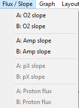
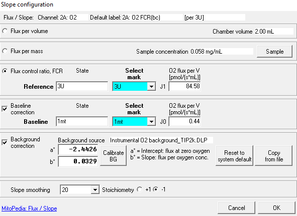
Flux / Slope is the time derivative of the signal. In DatLab, Flux / Slope is the name of the pull-down menu for (1) normalization of flux (chamber volume-specific flux, sample-specific flux or flow, or flux control ratios), (2) flux baseline correction, (3) Instrumental background oxygen flux, and (4) flux smoothing, selection of the scaling factor, and stoichiometric normalization using a stoichiometric coefficient. Before changing the normalization of flux from volume-specific flux to sample-specific flux or flow, or flux control ratios, please be sure to use the standard Layout 04a (Flux per volume) or 04b (Flux per volume overlay). When starting with the instrumental standard Layouts 1-3, which display the O2 slope negative, the sample-specific flux or flow, or flux control ratios will not be automatically background corrected. To obtain the background corrected specific flux or flux control ratios, it is needed to tick the background correction in the lower part of the slope configuration window. Background correction is especially critical when performing measurements in a high oxygen regime or using samples with a low respiratory flux or flow.
Abbreviation: J
Contributed by Cardoso Luiza HD, Gnaiger Erich 2020-03-04
Slope
- In an ideally closed chamber the external fluxes are zero, thus the concentration changes are exclusively due to (internal) transformations, which are chemical reactions. Then respiratory flux expressed per unit of chamber volume can be calculated from the slope of oxygen concentration over time (Gnaiger 2020).
Eq(1): X Slope neg = dcX/dt · νX-1 · SF | Units: [pmol/(s·mL)]
- For the oxygen channel, X=O2, cO2 is the oxygen concentration [nmol/mL = µmol/L = µM], dcO2/dt is the (positive) slope of oxygen concentration over time [nmol/(s · mL)], νO2-1 = -1 is the stoichiometric coefficient for the reaction of oxygen consumption (oxygen is removed in the chemical reaction, thus the stoichiometric coefficient is negative, expressing oxygen flux as the negative slope; Gnaiger 1993), and SF=1,000 is the scaling factor (converting units for the amount of oxygen from nmol to pmol).
- A Savitzky-Golay smoothing filter is used in DatLab as a basis for calculating the time derivative (Flux / Slope) of the signal (oxygen, fluorescence, ..).
- For each signal channel, the signal for the measured substance X is typically calibrated as an amount of substance concentration, cX [µM = nmol/mL]. The signal of the potentiometric channel, however, is primarily expressed logarithmically as pX=-log(cX/c°) and then transformed to cX. The slope is calculated as the change of concentration over time, dcX/dt [nmol· s-1· mL-1]. In a chemical reaction, the change of substance X is stoichiometrically related to the changes of all other substrates and products involved in the reaction. If the stoichiometry of the reaction is normalized for substance X, then its stoichiometric coefficient is unity and νX equals 1 if the substance is a product formed in the reaction, but νX equals -1 if the substance is a substrate consumed in the reaction. Oxygen is formed in photosynthesis and νX=1 when expressing photosynthesis as oxygen flux. Oxygen is consumed in aerobic respiration and νX=-1 when expressing respiration as oxygen flux.
Flux baseline correction
- If the sample itself introduces a constant flux in a baseline state (indicated as subscript 0), which is not considered to represent the metabolic reaction, then a flux baseline correction (bc) may be applied by subtracting the baseline flux, JV,0, from the total flux:
Eq(2b): JV,X(bc) = JV,X - JV,0 | Units: [pmol/(s·mL)]
O2 background correction
- In an experimentally closed chamber, external fluxes due to diffusion or convection into or out of the chamber are minimized, ideally to zero. Unavoidable external fluxes are corrected for, as there are side reactions due to the measuring system, such as oxygen consumption by the oxygen sensor or chemical background effects due to autoxidation of chemical components added to the medium. These external fluxes and side reactions of the experimental system are lumped together in the background flux, J°V,X. A Instrumental background oxygen flux is applied to the total slope, to obtain the metabolic flux, JV,X, describing the experimental reaction under investigation:
Eq(2a): JV,X = dcX/dt · νX-1 · SF - J°V,X | Units: [pmol/(s·mL)]
- J°V,O2 is the volume-specific background oxygen flux.
- In order to apply the instrumental O2 background values click on Calibrate BG button in the Slope configuration window. If the linearity, intercept (a°) and slope (b°) values are acceptable click on “Calibrate”. Apply the background correction by ticking the box “Background correction” and then press OK in the Slope configuration window. If this is done while DatLab is connected to the O2k, the information will be saved for the next experimental runs.
Copy from file
- If you did not apply an instrumental O2 background correction to your experimental DatLab file, you have the option to load the instrumental O2 background test parameters directly from the DLD file previously saved with the calibration by clicking on the Copy from file button in the Slope configuration window. Select your previously evaluated instrumental O2 background test file and load the parameters (i.e., intercept and slope) in DatLab.
Normalization
- Eqs(1) and (2) describe the dynamics of X per unit volume.
Eq(2a):  JV,X = X Slope neg - J°V,X  |  Units: [pmol/(s·mL)]
Eq(2b):  JV,X(bc) = JV,X - JV,0  |  Units: [pmol/(s·mL)]
- Normalization for the amount or concentration of sample yields metabolic flow per number of cells, IX, or specific metabolic flux per mass, Jm,X (unstructured analysis), or per mt-content (per mt-marker) in structured analysis (Gnaiger 2020).
Eq(3a): IX = JV,X/(106 cells/mL)  |  Units: [pmol/(s·106 cells)] = [amol/(s·cell)]
Eq(3b): IX(bc) = (JV,X - JV,0)/(106 cells/mL)  |  Units: [pmol/(s·106 cells)] = [amol/(s·cell)]
Eq(4a): Jm,X = JV,X/(mg/mL)  |  Units: [pmol/(s·mg)]
Eq(4b): Jm,X(bc) = (JV,X - JV,0)/(mg/mL)  |  Units: [pmol/(s·mg)]
Flux Control Ratio
- Flux control ratios are dimensionless, using a reference flux for normalization. The reference flux is determined in a metabolic reference state (1) as internal mt-marker (Gnaiger 2020),
Eq(5a): FCR = JV,X/JV,1
Eq(5b): FCR(bc) = (JV,X - JV,0)/(JV,1 - JV,0)
Smoothing, noise, and sample stability
- Recorded data: The default data recording interval is 2 s, applied with most SUIT protocols. The larger the data recording interval, the lower is the time resolution and the larger is the smoothing of flux.
- Smoothing in Flux / Slope: The default setting of Slope smoothing is 40 data points, i.e., 40 data points or an interval of 80 s at a data recording interval of 2 s are used for calculation of a non-linear fit, from which the slope is calculated for the current data point. 40 is used for O2 calibration and instrumental O2 background tests. 20 is recommended for data recording and analysis in typical SUIT experiments. When a larger noise is observed particularly in experiments with permeabilized muscle fibers, an increase to 25 displays more representative traces.
- Flux may decline over time, due to (1) loss of respiratory capacity within a respiratory state when the properties of the sample are not stable, (2) reversible oxygen limitation in the closed chamber, (3) an overshoot directly after re-oxygenation, or (4) a slow response to an inhibitor. Flux may increase over time due to (1) a slow response to the addition of ADP or a fuel substrate, or (2) an undershoot observed in rare cases after re-oxygenation. An extended time interval is required for recording flux in a particular respiratory state, if (1) flux increases over time (this may take >30 min, with a mark set at the final steady-state), and (2) flux shows high levels of noise (then 10 min may be required for setting a mark).
Flux analysis
- In a SUIT protocol each titration can be considered as a transition between a background state and a reference state, expressed as a flux control efficiency. A sequence of steady-state states can be analyzed in terms of flux control ratios, FCR, corrected for a common baseline, and normalized for flux in a common reference state. If a steady-state (constant) flux is not reached between sequential respiratory states induced by titrations, corrections for dynamic changes of flux as a function of time may be applied, else the conditions for steady-state analysis break down. In such cases, step analysis with continuous evaluation of a change of flux (second-time derivative) may provide the only reliable information. In reality, some noise or bias is included in steady-state analysis above a threshold level, below which such data sets would be excluded from the steady-state analysis.
O2
How to Analyze with DatLab 7.4
Previous versions of DatLab
Look for MiPNets and take information from DatLab-Analysis templates
H2O2
- Further information about hydrogen peroxide detection using Amplex UltraRed assay could be found under the page Amplex UltraRed
How to Analyze with DatLab 7.4
- Instruction to the Excel template for H2O2 flux analysis using Amplex UltraRed assay in MiR05-Kit: MiPNet24.10 Hydrogen peroxide flux analysis
- The calculations applied in the Excel template are provided here complying with Oroboros transparency policy and can be applied for measurements carried out in MiR05-Kit supplemented with DTPA:
- For details, see: Komlodi 2021 MitoFit AmR-O2
- 1. Calculation of background fluorescence slope of the Amplex UltraRed assay using MiR05-Kit supplemented with the iron chelator DTPA
- The background fluorescence slope Jamp,BGr [mV·s-1] was a linear function (proportional to the fluorescence signal Uamp [V]) in MiR05 with slope bamp and intercept aamp; bamp and aamp were determined for each Lot of MiR05-Kit.
Eq(1):Jamp,BGr = bamp·Uamp + aamp
- Linear dependence on fluorescence intensity Uamp [V] measured at the reference O2 concentration [O2]r which was close to air saturation
- 2. Linear dependence on O2 concentration described by the oxygen correction factor FO2,
Eq(2):FO2 = (0.0002 · [O2]e + 0.067)/(0.0002 · [O2]r + 0.067)
[O2]e is the experimental O2 concentration at a given respiratory state.
- 3. Oxygen-adjusted background fluorescence slope Jamp,BG [mV·s-1],
Eq(3) Jamp,BG = Jamp,BGr · FO2
- 4. Background-corrected experimental fluorescence slope Jamp,corr [mV·s-1] based on the experimental fluorescence slope in the presence of sample Jamp [mV·s-1] at [O2]e,
Eq(4) Jamp,corr = Jamp – Jamp,BG
- 5. Calibration for H2O2-sensitivity [V·µM-1] determined from H2O2 calibrations to obtain extracellular H2O2 flux JH2O2 [pmol·s-1·mL-1],
Eq(5) JV,H2O2 = Jamp,corr /sensitivity
- 6. Specific H2O2 flux JH2O2/X [pmol·s-1·x-1]
- Specific H2O2 flux is the flux corrected by the sample concentration. When using the Excel analysis template to calculate the H2O2 fluxes, be sure to check accordingly the following options: ‘ Titration volume correction’ and ‘Known sample concentration’. The specific H2O2 flux is given in the following unit [pmol·s-1·x-1], taking in consideration that the sample concentration is [x·mL-1]. The unit x can be substituted by the unit used in your project, e.g., a mg of protein or a million of cell.
Eq(6) JH2O2/X= JV,H2O2/(SCF·CX0)
· SCF: sample concentration correction factor
· CX0: initial sample concentration in the chamber [x·mL-1]
- - If ‘titration volume correction’ option is not enabled: sample concentration correction factor = 1
- - If ‘Known sample concentration’ is unchecked: [sample] = 1 [x·mL-1]
- - The calculation of the sample concentration correction factor is the same used for the calculation of the specific oxygen flux (See: MiPNet24.06 Oxygen flux analysis - DatLab 7.4
- 7. Baseline-corrected specific H2O2 flux (bc) JH2O2/X(bc) [pmol·s-1·x-1]
- The baseline state is pre-set for each SUIT protocol available at the template.
Eq(7):JH2O2/X(bc)=JH2O2/X-JH2O2/Xbaseline
- 8. Specific H2O2 flux/Specific O2 flux ratio
- The H2O2 flux/O2 flux ratio gives us information about the relative contribution of H2O2 production relating to the respiration, or other words, how much oxygen of total oxygen turned over is consumed for H2O2 generation.
Eq(8):JH2O2/X/JO2/X
- The specific fluxes corrected for the baseline are not used for this ratio, because the baseline state for H2O2 flux and O2 flux calculations might be different depending on the protocol.
Troubleshooting
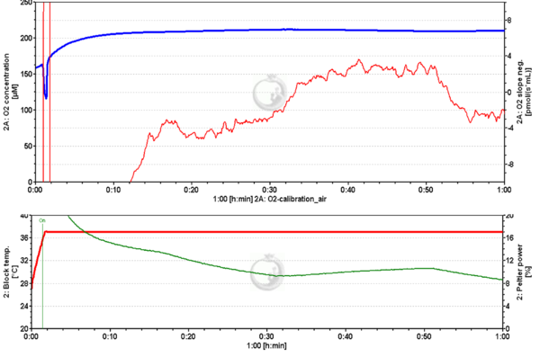
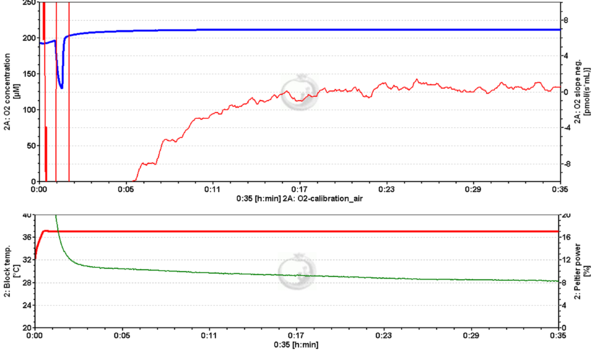
Oxygen slope neg. fluctuating
- Customer ID: Anonymous
- Question: I am having some trouble getting the O2 slope neg. to stabilize at zero pmol/(s•mL) during air calibration. The signal will be stable at -4 pmol/(s•mL), then fairly quickly climb to +4 pmol/(s•mL) then swap back down to -4 pmol/(s•mL) in a long wave that repeats periodically over time.
- Answer: We noticed that your Peltier power follows the changes observed in the O2 slope neg. To rule out electrical fluctuations we would ask you to exchange the energy supply of the O2k and run an air calibration file to check.
- After changing the electrical supply the O2 slope neg. and the Peltier power signal were stable.
References
- Gnaiger E (1993) Nonequilibrium thermodynamics of energy transformations. Pure Appl Chem 65:1983-2002. - »Bioblast link«
- Gnaiger E (2020) Mitochondrial pathways and respiratory control. An introduction to OXPHOS analysis. 5th ed. Bioenerg Commun:112 pp. - »Bioblast link«
- Press WH, Teukolsky SA (1990) Savitzky-Golay smoothing filters. Computers in Physics Nov/Dec 1990:669-72. - »Bioblast link«
Further links
MitoPedia methods: Respirometry, Fluorometry
MitoPedia O2k and high-resolution respirometry:
DatLab

